Heterogeneous graphs and DeepSNAP
From colab 5
In this Colab, we will shift our focus from homogenous graphs to heterogeneous graphs. Heterogeneous graphs extend the traditional homogenous graphs that we have been working with by incorperating different node and edge types. This additional information allows us to extend the graph neural nework models that we have worked with before. Namely, we can apply heterogenous message passing, where different message types now exist between different node and edge type relationships.
In this notebook, we will first learn how to transform NetworkX graphs into DeepSNAP representations. Then, we will dive deeper into how DeepSNAP stores and represents heterogeneous graphs as PyTorch Tensors.
Lastly, we will build our own heterogenous graph neural netowrk models using PyTorch Geometric and DeepSNAP. We will then apply our models for a node property prediction task; specifically, we will evaluate these models on the heterogeneous ACM node prediction dataset.
Note: Make sure to sequentially run all the cells in each section, so that the intermediate variables / packages will carry over to the next cell
Have fun and good luck on Colab 5 :)
Device
You might need to use GPU for this Colab.
Please click Runtime and then Change runtime type. Then set the hardware accelerator to GPU.
Installation
[ ]:
# Install torch geometric
import os
if 'IS_GRADESCOPE_ENV' not in os.environ:
  !pip install torch-scatter -f https://data.pyg.org/whl/torch-1.10.0+cu111.html
  !pip install torch-sparse -f https://data.pyg.org/whl/torch-1.10.0+cu111.html
  !pip install torch-geometric
  !pip install -q git+https://github.com/snap-stanford/deepsnap.git
  !pip install -U -q PyDrive
Looking in links: https://data.pyg.org/whl/torch-1.10.0+cu111.html
Collecting torch-scatter
  Downloading https://data.pyg.org/whl/torch-1.10.0%2Bcu113/torch_scatter-2.0.9-cp37-cp37m-linux_x86_64.whl (7.9 MB)
     |████████████████████████████████| 7.9 MB 4.2 MB/s
Installing collected packages: torch-scatter
Successfully installed torch-scatter-2.0.9
Looking in links: https://data.pyg.org/whl/torch-1.10.0+cu111.html
Collecting torch-sparse
  Downloading https://data.pyg.org/whl/torch-1.10.0%2Bcu113/torch_sparse-0.6.13-cp37-cp37m-linux_x86_64.whl (3.5 MB)
     |████████████████████████████████| 3.5 MB 4.0 MB/s
Requirement already satisfied: scipy in /usr/local/lib/python3.7/dist-packages (from torch-sparse) (1.4.1)
Requirement already satisfied: numpy>=1.13.3 in /usr/local/lib/python3.7/dist-packages (from scipy->torch-sparse) (1.21.6)
Installing collected packages: torch-sparse
Successfully installed torch-sparse-0.6.13
Collecting torch-geometric
  Downloading torch_geometric-2.0.4.tar.gz (407 kB)
     |████████████████████████████████| 407 kB 3.8 MB/s
Requirement already satisfied: tqdm in /usr/local/lib/python3.7/dist-packages (from torch-geometric) (4.64.0)
Requirement already satisfied: numpy in /usr/local/lib/python3.7/dist-packages (from torch-geometric) (1.21.6)
Requirement already satisfied: scipy in /usr/local/lib/python3.7/dist-packages (from torch-geometric) (1.4.1)
Requirement already satisfied: pandas in /usr/local/lib/python3.7/dist-packages (from torch-geometric) (1.3.5)
Requirement already satisfied: jinja2 in /usr/local/lib/python3.7/dist-packages (from torch-geometric) (2.11.3)
Requirement already satisfied: requests in /usr/local/lib/python3.7/dist-packages (from torch-geometric) (2.23.0)
Requirement already satisfied: pyparsing in /usr/local/lib/python3.7/dist-packages (from torch-geometric) (3.0.8)
Requirement already satisfied: scikit-learn in /usr/local/lib/python3.7/dist-packages (from torch-geometric) (1.0.2)
Requirement already satisfied: MarkupSafe>=0.23 in /usr/local/lib/python3.7/dist-packages (from jinja2->torch-geometric) (2.0.1)
Requirement already satisfied: pytz>=2017.3 in /usr/local/lib/python3.7/dist-packages (from pandas->torch-geometric) (2022.1)
Requirement already satisfied: python-dateutil>=2.7.3 in /usr/local/lib/python3.7/dist-packages (from pandas->torch-geometric) (2.8.2)
Requirement already satisfied: six>=1.5 in /usr/local/lib/python3.7/dist-packages (from python-dateutil>=2.7.3->pandas->torch-geometric) (1.15.0)
Requirement already satisfied: certifi>=2017.4.17 in /usr/local/lib/python3.7/dist-packages (from requests->torch-geometric) (2021.10.8)
Requirement already satisfied: urllib3!=1.25.0,!=1.25.1,<1.26,>=1.21.1 in /usr/local/lib/python3.7/dist-packages (from requests->torch-geometric) (1.24.3)
Requirement already satisfied: chardet<4,>=3.0.2 in /usr/local/lib/python3.7/dist-packages (from requests->torch-geometric) (3.0.4)
Requirement already satisfied: idna<3,>=2.5 in /usr/local/lib/python3.7/dist-packages (from requests->torch-geometric) (2.10)
Requirement already satisfied: joblib>=0.11 in /usr/local/lib/python3.7/dist-packages (from scikit-learn->torch-geometric) (1.1.0)
Requirement already satisfied: threadpoolctl>=2.0.0 in /usr/local/lib/python3.7/dist-packages (from scikit-learn->torch-geometric) (3.1.0)
Building wheels for collected packages: torch-geometric
  Building wheel for torch-geometric (setup.py) ... done
  Created wheel for torch-geometric: filename=torch_geometric-2.0.4-py3-none-any.whl size=616603 sha256=618f6e77ed5dfbb624ad5e3008a86fd6ca223dbd6c0ada51268ba48fcf858f4a
  Stored in directory: /root/.cache/pip/wheels/18/a6/a4/ca18c3051fcead866fe7b85700ee2240d883562a1bc70ce421
Successfully built torch-geometric
Installing collected packages: torch-geometric
Successfully installed torch-geometric-2.0.4
  Building wheel for deepsnap (setup.py) ... done
[ ]:
if 'IS_GRADESCOPE_ENV' not in os.environ:
  !nvcc --version
  !python -c "import torch; print(torch.version.cuda)"
nvcc: NVIDIA (R) Cuda compiler driver
Copyright (c) 2005-2020 NVIDIA Corporation
Built on Mon_Oct_12_20:09:46_PDT_2020
Cuda compilation tools, release 11.1, V11.1.105
Build cuda_11.1.TC455_06.29190527_0
11.3
[2]:
import os
if 'IS_GRADESCOPE_ENV' not in os.environ:
  import torch
  print(torch.__version__)
  import torch_geometric
  print(torch_geometric.__version__)
1.11.0
2.0.4
DeepSNAP Basics
In previous Colabs we used both of graph class (NetworkX) and tensor (PyG) representations of graphs separately. The graph class nx.Graph provides rich analysis and manipulation functionalities, such as the clustering coefficient and PageRank. To feed the graph into the model, we need to transform the graph into tensor representations including edge tensor edge_index and node attributes tensors x and y. But only using tensors (as the graphs formatted in PyG datasets and
data) will make many graph manipulations and analysis less efficient and harder. So, in this Colab we will use DeepSNAP which combines both representations and offers a full pipeline for GNN training / validation / testing.
In general, DeepSNAP is a Python library to assist efficient deep learning on graphs. DeepSNAP features in its support for flexible graph manipulation, standard pipeline, heterogeneous graphs and simple API.
DeepSNAP is easy to be used for the sophisticated graph manipulations, such as feature computation, pretraining, subgraph extraction etc. during/before the training.
In most frameworks, standard pipelines for node, edge, link, graph-level tasks under inductive or transductive settings are left to the user to code. In practice, there are additional design choices involved (such as how to split dataset for link prediction). DeepSNAP provides such a standard pipeline that greatly saves repetitive coding efforts, and enables fair comparision for models.
Many real-world graphs are heterogeneous graphs. But packages support for heterogeneous graphs, including data storage and flexible message passing, is lacking. DeepSNAP provides an efficient and flexible heterogeneous graph that supports both the node and edge heterogeneity.
DeepSNAP is a newly released project and it is still under development. If you find any bugs or have any improvement ideas, feel free to raise issues or create pull requests on the GitHub directly :)
In this Colab, we will focus on learning using Heterogeneous Graphs. Not many libraries are able to handle heterogeneous graphs, but DeepSNAP handles them quite elegantly, which is why we’re introducing it here!
1) DeepSNAP Heterogeneous Graph
First, we will explore how to transform a NetworkX graph into the format supported by DeepSNAP.
In DeepSNAP we have three levels of attributes. We can have node level attributes including node_feature and node_label. The other two levels of attributes are graph and edge attributes. The usage is similar to the node level one except that the feature becomes edge_feature or graph_feature and label becomes edge_label or graph_label etc.
node_feature: The feature of each node (torch.tensor) * edge_feature: The feature of each edge (torch.tensor) * node_label: The label of each node (int) * node_type: The node type of each node (string) * edge_type: The edge type of each edge (string)where the key new features we add are node_type and edge_type, which enables us to perform heterogenous message passing.
For this first question we will work with the familiar karate club graph seen in Colab 1. To start, since each node in the graph belongs to one of two clubs (club “Mr. Hi” or club “Officer”), we will treat the club as the node_type. The code below demonstrates how to differentiate the nodes in the NetworkX graph.
[3]:
import networkx as nx
from networkx.algorithms.community import greedy_modularity_communities
import matplotlib.pyplot as plt
import copy

if 'IS_GRADESCOPE_ENV' not in os.environ:
  from pylab import show
  G = nx.karate_club_graph()
  community_map = {}
  for node in G.nodes(data=True):
    if node[1]["club"] == "Mr. Hi":
      community_map[node[0]] = 0
    else:
      community_map[node[0]] = 1
  node_color = []
  color_map = {0: 0, 1: 1}
  node_color = [color_map[community_map[node]] for node in G.nodes()]
  pos = nx.spring_layout(G)
  plt.figure(figsize=(7, 7))
  nx.draw(G, pos=pos, cmap=plt.get_cmap('coolwarm'), node_color=node_color)
  show()

Question 1.1: Assigning Node Type and Node Features
Using the community_map dictionary and graph G from above, add node attributes node_type and node_label to the graph G. Namely, for node_type assign nodes in the “Mr. Hi” club to a node type n0 and nodes in club “Officer” a node type n1. Note: the node type should be a string property.
Then for node_label, assign nodes in “Mr. Hi” club to a node_label 0 and nodes in club “Officer” a node_label of 1.
Lastly, assign every node the tensor feature vector \([1, 1, 1, 1, 1]\).
Hint: Look at the NetworkX function nx.classes.function.set_node_attributes.
Note: This question is not specifically graded but is important for later questions.
[4]:
import torch

def assign_node_types(G, community_map):
  # TODO: Implement a function that takes in a NetworkX graph
  # G and community map assignment (mapping node id --> 0/1 label)
  # and adds 'node_type' as a node_attribute in G.

  ############# Your code here ############
  ## (~2 line of code)
  ## Note
  ## 1. Look up NetworkX `nx.classes.function.set_node_attributes`
  ## 2. Look above for the two node type values!

  values = {}
  for node in G.nodes(data=True):
      if community_map[node[0]] == 0:
          values[node[0]] = 'n0'
      else:
          values[node[0]] = 'n1'
  nx.classes.function.set_node_attributes(G, values, name='node_type')

  #########################################

def assign_node_labels(G, community_map):
  # TODO: Implement a function that takes in a NetworkX graph
  # G and community map assignment (mapping node id --> 0/1 label)
  # and adds 'node_label' as a node_attribute in G.

  ############# Your code here ############
  ## (~2 line of code)
  ## Note
  ## 1. Look up NetworkX `nx.classes.function.set_node_attributes`

  nx.classes.function.set_node_attributes(G, community_map, name='node_label')

  #########################################

def assign_node_features(G):
  # TODO: Implement a function that takes in a NetworkX graph
  # G and adds 'node_feature' as a node_attribute in G. Each node
  # in the graph has the same feature vector - a torchtensor with
  # data [1., 1., 1., 1., 1.]

  ############# Your code here ############
  ## (~2 line of code)
  ## Note
  ## 1. Look up NetworkX `nx.classes.function.set_node_attributes`

  nx.classes.function.set_node_attributes(G, [1., 1., 1., 1., 1.], name='node_feature')

  #########################################

if 'IS_GRADESCOPE_ENV' not in os.environ:
  assign_node_types(G, community_map)
  assign_node_labels(G, community_map)
  assign_node_features(G)

  # Explore node properties for the node with id: 20
  node_id = 20
  print (f"Node {node_id} has properties:", G.nodes(data=True)[node_id])
Node 20 has properties: {'club': 'Officer', 'node_type': 'n1', 'node_label': 1, 'node_feature': [1.0, 1.0, 1.0, 1.0, 1.0]}
Question 1.2: Assigning Edge Types
Next, we will assign three different edge_types: * Edges within club “Mr. Hi”: e0 * Edges within club “Officer”: e1 * Edges between the two clubs: e2
Hint: Use the community_map from before and nx.classes.function.set_edge_attributes
[5]:
def assign_edge_types(G, community_map):
  # TODO: Implement a function that takes in a NetworkX graph
  # G and community map assignment (mapping node id --> 0/1 label)
  # and adds 'edge_type' as a edge_attribute in G.

  ############# Your code here ############
  ## (~5 line of code)
  ## Note
  ## 1. Create an edge assignment dict following rules above
  ## 2. Look up NetworkX `nx.classes.function.set_edge_attributes`

  values = {}
  for edge in G.edges(data=True):
    if community_map[edge[0]] == 0 and community_map[edge[1]] == 0:
      values[(edge[0], edge[1])] = 'e0'
    elif community_map[edge[0]] == 1 and community_map[edge[1]] == 1:
      values[(edge[0], edge[1])] = 'e1'
    else:
      values[(edge[0], edge[1])] = 'e2'
  nx.classes.function.set_edge_attributes(G, values, name='edge_type')

  #########################################

if 'IS_GRADESCOPE_ENV' not in os.environ:
  assign_edge_types(G, community_map)

  # Explore edge properties for a sampled edge and check the corresponding
  # node types
  edge_idx = 15
  n1 = 0
  n2 = 31
  edge = list(G.edges(data=True))[edge_idx]
  print (f"Edge ({edge[0]}, {edge[1]}) has properties:", edge[2])
  print (f"Node {n1} has properties:", G.nodes(data=True)[n1])
  print (f"Node {n2} has properties:", G.nodes(data=True)[n2])
Edge (0, 31) has properties: {'edge_type': 'e2'}
Node 0 has properties: {'club': 'Mr. Hi', 'node_type': 'n0', 'node_label': 0, 'node_feature': [1.0, 1.0, 1.0, 1.0, 1.0]}
Node 31 has properties: {'club': 'Officer', 'node_type': 'n1', 'node_label': 1, 'node_feature': [1.0, 1.0, 1.0, 1.0, 1.0]}
Heterogeneous Graph Visualization
Now we can visualize the Heterogeneous Graph we have generated.
[6]:
if 'IS_GRADESCOPE_ENV' not in os.environ:
  edge_color = {}
  for edge in G.edges():
    n1, n2 = edge
    edge_color[edge] = community_map[n1] if community_map[n1] == community_map[n2] else 2
    if community_map[n1] == community_map[n2] and community_map[n1] == 0:
      edge_color[edge] = 'blue'
    elif community_map[n1] == community_map[n2] and community_map[n1] == 1:
      edge_color[edge] = 'red'
    else:
      edge_color[edge] = 'green'

  G_orig = copy.deepcopy(G)
  nx.classes.function.set_edge_attributes(G, edge_color, name='color')
  colors = nx.get_edge_attributes(G,'color').values()
  labels = nx.get_node_attributes(G, 'node_type')
  plt.figure(figsize=(8, 8))
  nx.draw(G, pos=pos, cmap=plt.get_cmap('coolwarm'), node_color=node_color, edge_color=colors, labels=labels, font_color='white')
  show()

where we differentiate edges within each clubs (2 types) and edges between the two clubs (1 type). Different types of nodes and edges are visualized in different colors. The NetworkX object G in following code can be transformed into deepsnap.hetero_graph.HeteroGraph directly.
Transforming to DeepSNAP representation
We will now work through transforming the NetworkX object G into a deepsnap.hetero_graph.HeteroGraph.
[9]:
from deepsnap.hetero_graph import HeteroGraph

if 'IS_GRADESCOPE_ENV' not in os.environ:
  hete = HeteroGraph(G_orig)
Question 1.3: How many nodes are of each type (10 Points)
[10]:
def get_nodes_per_type(hete):
  # TODO: Implement a function that takes a DeepSNAP dataset object
  # and return the number of nodes per `node_type`.

  num_nodes_n0 = 0
  num_nodes_n1 = 0

  ############# Your code here ############
  ## (~2 line of code)
  ## Note
  ## 1. Colab autocomplete functionality might be useful.

  num_nodes_n0 = hete.num_nodes('n0')
  num_nodes_n1 = hete.num_nodes('n1')

  #########################################

  return num_nodes_n0, num_nodes_n1

if 'IS_GRADESCOPE_ENV' not in os.environ:
  num_nodes_n0, num_nodes_n1 = get_nodes_per_type(hete)
  print("Node type n0 has {} nodes".format(num_nodes_n0))
  print("Node type n1 has {} nodes".format(num_nodes_n1))
Node type n0 has 17 nodes
Node type n1 has 17 nodes
Question 1.4: Message Types - How many edges are of each message type (10 Points)
When working with heterogenous graphs, as we have discussed before, we now work with heterogenous message types (i.e. different message types for the different node_type and edge_type combinations). For example, an edge of type e0 connecting two nodes in club “Mr. HI” would have a message type of (n0, e0, n0). In this problem we will analyze how many edges in our graph are of each message type.
Hint: If you want to learn more about what the different message types are try the call hete.message_types
[11]:
def get_num_message_edges(hete):
  # TODO: Implement this function that takes a DeepSNAP dataset object
  # and return the number of edges for each message type.
  # You should return a list of tuples as
  # (message_type, num_edge)

  message_type_edges = []

  ############# Your code here ############
  ## (~2 line of code)
  ## Note
  ## 1. Colab autocomplete functionality might be useful.

  for message_type in hete.message_types:
      message_type_edges.append([message_type, hete.num_edges(message_type=message_type)])

  #########################################

  return message_type_edges

if 'IS_GRADESCOPE_ENV' not in os.environ:
  message_type_edges = get_num_message_edges(hete)
  for (message_type, num_edges) in message_type_edges:
    print("Message type {} has {} edges".format(message_type, num_edges))
Message type ('n0', 'e0', 'n0') has 35 edges
Message type ('n0', 'e2', 'n1') has 11 edges
Message type ('n1', 'e1', 'n1') has 32 edges
Question 1.5: Dataset Splitting - How many nodes are in each dataset split? (10 Points)
DeepSNAP has built in Dataset creation and splitting methods for heterogeneous graphs. Here we will create train, validation, and test datasets for a node prediction task and inspect the resulting subgraphs. Specifically, write a function that computes the number of nodes with a known label in each dataset split.
[12]:
from deepsnap.dataset import GraphDataset

def compute_dataset_split_counts(datasets):
  # TODO: Implement a function that takes a dict of datasets in the form
  # {'train': dataset_train, 'val': dataset_val, 'test': dataset_test}
  # and returns a dict mapping dataset names to the number of labeled
  # nodes used for supervision in that respective dataset.

  data_set_splits = {}

  ############# Your code here ############
  ## (~3 line of code)
  ## Note
  ## 1. The DeepSNAP `node_label_index` dictionary will be helpful.
  ## 2. Remember to count both node_types
  ## 3. Remember each dataset only has one graph that we need to access
  ##    (i.e. dataset[0])

  for split in datasets.keys():
    data_set_splits[split] = len(datasets[split][0].node_label_index['n0']) + len(datasets[split][0].node_label_index['n1'])

  #########################################

  return data_set_splits

if 'IS_GRADESCOPE_ENV' not in os.environ:
  dataset = GraphDataset([hete], task='node')
  # Splitting the dataset
  dataset_train, dataset_val, dataset_test = dataset.split(transductive=True, split_ratio=[0.4, 0.3, 0.3])
  datasets = {'train': dataset_train, 'val': dataset_val, 'test': dataset_test}

  data_set_splits = compute_dataset_split_counts(datasets)
  for dataset_name, num_nodes in data_set_splits.items():
    print("{} dataset has {} nodes".format(dataset_name, num_nodes))
train dataset has 12 nodes
val dataset has 10 nodes
test dataset has 12 nodes
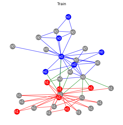
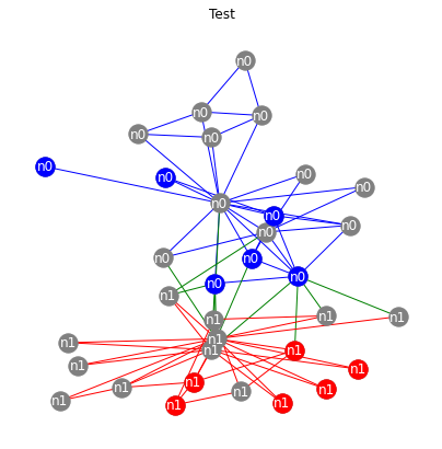
DeepSNAP Dataset Visualization
We can now visualize the different nodes and edges used in each graph dataset split.
[13]:
from deepsnap.dataset import GraphDataset

if 'IS_GRADESCOPE_ENV' not in os.environ:
  dataset = GraphDataset([hete], task='node')
  # Splitting the dataset
  dataset_train, dataset_val, dataset_test = dataset.split(transductive=True, split_ratio=[0.4, 0.3, 0.3])
  titles = ['Train', 'Validation', 'Test']

  for i, dataset in enumerate([dataset_train, dataset_val, dataset_test]):
    n0 = hete._convert_to_graph_index(dataset[0].node_label_index['n0'], 'n0').tolist()
    n1 = hete._convert_to_graph_index(dataset[0].node_label_index['n1'], 'n1').tolist()

    plt.figure(figsize=(7, 7))
    plt.title(titles[i])
    nx.draw(G_orig, pos=pos, node_color="grey", edge_color=colors, labels=labels, font_color='white')
    nx.draw_networkx_nodes(G_orig.subgraph(n0), pos=pos, node_color="blue")
    nx.draw_networkx_nodes(G_orig.subgraph(n1), pos=pos, node_color="red")
    show()

2) Heterogeneous Graph Node Property Prediction
Now, we will use PyTorch Geometric and DeepSNAP to implement a GNN model for heterogeneous graph node property prediction (node classification). We will draw upon our understanding of heterogeneous graphs from lecture and previous work in implementing GNN layers using PyG (introduced in Colab 3).
First let’s take a look at the general structure of a heterogeneous GNN layer by working through an example:
Let’s assume we have a graph \(G\), which contains two node types \(a\) and \(b\), and three message types \(m_1=(a, r_1, a)\), \(m_2=(a, r_2, b)\) and \(m_3=(a, r_3, b)\). Note: during message passing we view each message as (src, relation, dst), where messages “flow” from src to dst node types. For example, during message passing, updating node type \(b\) relies on two different message types \(m_2\) and \(m_3\).
When applying message passing in heterogenous graphs, we seperately apply message passing over each message type. Therefore, for the graph \(G\), a heterogeneous GNN layer contains three seperate Heterogeneous Message Passing layers (HeteroGNNConv in this Colab), where each HeteroGNNConv layer performs message passing and aggregation with respect to only one message type. Since a message type is viewed as (src, relation, dst) and messages “flow” from src to dst, each
HeteroGNNConv layer only computes embeddings for the dst nodes of a given message type. For example, the HeteroGNNConv layer for message type \(m_2\) outputs updated embedding representations only for node’s with type b.
An overview of the heterogeneous layer we will create is shown below:
where we highlight the following notation:
\(H_a^{(l)[m_1]}\) is the intermediate matrix of of node embeddings for node type \(a\), generated by the \(l\)th
HeteroGNNConvlayer for message type \(m_1\).\(H_a^{(l)}\) is the matrix with current embeddings for nodes of type \(a\) after the \(l\)th layer of our Heterogeneous GNN model. Note that these embeddings can rely on one or more intermediate
HeteroGNNConvlayer embeddings(i.e. \(H_b^{(l)}\) combines \(H_b^{(l)[m_2]}\) and \(H_b^{(l)[m_3]}\)).
Since each HeteroGNNConv is only applied over a single message type, we additionally define a Heterogeneous GNN Wrapper layer (HeteroGNNWrapperConv). This wrapper manages and combines the output of each HeteroGNNConv layer in order to generate the complete updated node embeddings for each node type in layer \(l\) of our model. More specifically, the \(l^{th}\) HeteroGNNWrapperConv layer takes as input the node embeddings computed for each message type and node type (e.g.
\(H_b^{(l)[m_2]}\) and \(H_b^{(l)[m_3]}\)) and aggregates across message types with the same \(dst\) node type. The resulting output of the \(l^{th}\) HeteroGNNWrapperConv layer is the updated embedding matrix \(H_i^{(l)}\) for each node type i.
Continuing on our example above, to compute the node embeddings \(H_b^{(l)}\) the wrapper layer aggregates output embeddings from the HeteroGNNConv layers associated with message types \(m_2\) and \(m_3\) (i.e. \(H_b^{(l)[m_2]}\) and \(H_b^{(l)[m_3]}\)).
With the HeteroGNNWrapperConv module, we can now draw a “simplified” heterogeneous layer structure as follows:

NOTE: As reference, it may be helpful to additionally read through PyG’s introduciton to heterogeneous graph representations and buidling heterogeneous GNN models: https://pytorch-geometric.readthedocs.io/en/latest/notes/heterogeneous.html
Looking ahead, we recommend you implement the heterogeneous GNN model in following steps:
Implement
HeteroGNNConv.Implement just
meanaggregation withinHeteroGNNWrapperConv.Implement
generate_convs.Implement the
HeteroGNNmodel and thetrainfunction.Train the model with
meanaggregation and test your model to make sure your model has reasonable performance.Once you are confident in your mean aggregation model, implement
attnaggregation inHeteroGNNWrapperConv.Train the model with
attnaggregation and test your model to make sure your model has reasonable performance.
Note: The key point of advice is to work completely through implementing the mean aggregation heterogeneous GNN model before diving into the more difficult attention based model.
Setup
[14]:
import copy
import torch
import deepsnap
import numpy as np
import torch.nn as nn
import torch.nn.functional as F
import torch_geometric.nn as pyg_nn

from sklearn.metrics import f1_score
from deepsnap.hetero_gnn import forward_op
from deepsnap.hetero_graph import HeteroGraph
from torch_sparse import SparseTensor, matmul
Dataset
You need to login to your Google account and enter the verification code below.
[ ]:
if 'IS_GRADESCOPE_ENV' not in os.environ:
  from pydrive.auth import GoogleAuth
  from pydrive.drive import GoogleDrive
  from google.colab import auth
  from oauth2client.client import GoogleCredentials

  # Authenticate and create the PyDrive client
  auth.authenticate_user()
  gauth = GoogleAuth()
  gauth.credentials = GoogleCredentials.get_application_default()
  drive = GoogleDrive(gauth)
[ ]:
if 'IS_GRADESCOPE_ENV' not in os.environ:
  id='1ivlxd6lJMcZ9taS44TMGG72x2V1GeVvk'
  downloaded = drive.CreateFile({'id': id})
  downloaded.GetContentFile('acm.pkl')
Implementing HeteroGNNConv
Now let’s start working on our own implementation of the heterogeneous message passing layer (HeteroGNNConv)! Just as in Colabs 3 and 4, we will implement the layer using PyTorch Geometric.
At a high level, the HeteroGNNConv layer is equivalent to the homogenous GNN layers we implemented in Colab 3, but now applied to an individual heterogeous message type. Moreover, our heterogeneous GNN layer draws directly from the GraphSAGE message passing model (Hamilton et al. (2017)).
We begin by defining the HeteroGNNConv layer with respect to message type \(m\):
\begin{equation} m =(s, r, d) \end{equation}
where each message type is a tuple containing three elements: \(s\) - the source node type, \(r\) - the edge (relation) type, and \(d\) - the destination node type.
The message passing update rule that we implement is very similar to that of GraphSAGE, except we now need to include the node types and the edge relation type. The update rule for message type \(m\) is described below: s \begin{equation} h_v^{(l)[m]} = W^{(l)[m]} \cdot \text{CONCAT} \Big( W_d^{(l)[m]} \cdot h_v^{(l-1)}, W_s^{(l)[m]} \cdot AGG(\{h_u^{(l-1)}, \forall u \in N_{m}(v) \})\Big) \end{equation}
where we compute \(h_v^{(l)[m]}\), the node embedding representation for node \(v\) after HeteroGNNConv layer \(l\) with respect message type \(m\). Further unpacking the forumla we have: - \(W_s^{(l)[m]}\) - linear transformation matrix for the messages of neighboring source nodes of type \(s\) along message type \(m\). - \(W_d^{(l)[m]}\) - linear transformation matrix for the message from the node \(v\) itself of type \(d\). - \(W^{(l)[m]}\) -
linear transformation matrix for the concatenated messages from neighboring node’s and the central node. - \(h_u^{(l-1)}\) - the hidden embedding representation for node \(u\) after the \((l-1)\)th HeteroGNNWrapperConv layer. Note, that this embedding is not associated with a particular message type (see layer diagrams above). - \(N_{m}(v)\) - the set of neighbor source nodes \(s\) for the node v that we are embedding along message type \(m = (s, r, d)\).
NOTE: We emphasize that each weight matrix is associated with a specific message type \([m]\) and additionally, the weight matrices applied to node messages are differentiated by node type (i.e. \(W_s\) and \(W_d\)).
Lastly, for simplicity, we use mean aggregations for \(AGG\) where:
\begin{equation} AGG(\{h_u^{(l-1)}, \forall u \in N_{m}(v) \}) = \frac{1}{|N_{m}(v)|} \sum_{u\in N_{m}(v)} h_u^{(l-1)} \end{equation}
[42]:
class HeteroGNNConv(pyg_nn.MessagePassing):
    def __init__(self, in_channels_src, in_channels_dst, out_channels):
        super(HeteroGNNConv, self).__init__(aggr="mean")

        self.in_channels_src = in_channels_src
        self.in_channels_dst = in_channels_dst
        self.out_channels = out_channels

        # To simplify implementation, please initialize both self.lin_dst
        # and self.lin_src out_features to out_channels
        self.lin_dst = None
        self.lin_src = None

        self.lin_update = None

        ############# Your code here #############
        ## (~3 lines of code)
        ## Note:
        ## 1. Initialize the 3 linear layers.
        ## 2. Think through the connection between the mathematical
        ##    definition of the update rule and torch linear layers!

        self.lin_dst = nn.Linear(self.in_channels_src, self.out_channels)
        self.lin_src = nn.Linear(self.in_channels_dst, self.out_channels)
        self.lin_update = nn.Linear(2*self.out_channels, self.out_channels)

        ##########################################

    def forward(
        self,
        node_feature_src,
        node_feature_dst,
        edge_index,
        size=None
    ):
        ############# Your code here #############
        ## (~1 line of code)
        ## Note:
        ## 1. Unlike Colabs 3 and 4, we just need to call self.propagate with
        ## proper/custom arguments.

        return self.propagate(edge_index, node_feature_src=node_feature_src,
                    node_feature_dst=node_feature_dst, size=size)

        ##########################################

    def message_and_aggregate(self, edge_index, node_feature_src):

        out = None
        ############# Your code here #############
        ## (~1 line of code)
        ## Note:
        ## 1. Different from what we implemented in Colabs 3 and 4, we use message_and_aggregate
        ##    to combine the previously seperate message and aggregate functions.
        ##    The benefit is that we can avoid materializing x_i and x_j
        ##    to make the implementation more efficient.
        ## 2. To implement efficiently, refer to PyG documentation for message_and_aggregate
        ##    and sparse-matrix multiplication:
        ##    https://pytorch-geometric.readthedocs.io/en/latest/notes/sparse_tensor.html
        ## 3. Here edge_index is torch_sparse SparseTensor. Although interesting, you
        ##    do not need to deeply understand SparseTensor represenations!
        ## 4. Conceptually, think through how the message passing and aggregation
        ##    expressed mathematically can be expressed through matrix multiplication.

        out = matmul(edge_index, node_feature_src, reduce='mean')


        ##########################################

        return out

    def update(self, aggr_out, node_feature_dst):

        ############# Your code here #############
        ## (~4 lines of code)
        ## Note:
        ## 1. The update function is called after message_and_aggregate
        ## 2. Think through the one-one connection between the mathematical update
        ##    rule and the 3 linear layers defined in the constructor.

        dst_out = self.lin_dst(node_feature_dst)
        aggr_out = self.lin_src(aggr_out)
        # print(aggr_out.shape, dst_out.shape)
        aggr_out = torch.cat([dst_out, aggr_out], -1)
        # print(aggr_out.shape, )
        aggr_out = self.lin_update(aggr_out)

        ##########################################

        return aggr_out
Heterogeneous GNN Wrapper Layer
After implementing the HeteroGNNConv layer for each message type, we need to manage and aggregate the node embedding results (with respect to each message types). Here we will implement two types of message type level aggregation.
The first one is simply mean aggregation over message types:
\begin{equation} h_v^{(l)} = \frac{1}{M}\sum_{m=1}^{M}h_v^{(l)[m]} \end{equation}
where node \(v\) has node type \(d\) and we sum over the \(M\) message types that have destination node type \(d\). From our original example, for a node v of type \(b\) we aggregate v’s HeteroGNNConv embeddings for message types \(m_2\) and \(m_3\) (i.e. \(h_v^{(l)[m_2]}\) and \(h_v^{(l)[m_3]}\)).
The second method we implement is the semantic level attention introduced in HAN (Wang et al. (2019)). Instead of directly averaging on the message type aggregation results, we use attention to learn which message type result is more important, then aggregate across all the message types. Below are the equations for semantic level attention:
\begin{equation} e_{m} = \frac{1}{|V_{d}|} \sum_{v \in V_{d}} q_{attn}^T \cdot tanh \Big( W_{attn}^{(l)} \cdot h_v^{(l)[m]} + b \Big) \end{equation}
where \(m\) is the message type and \(d\) refers to the destination node type for that message (\(m = (s, r, d)\)). Additionally, \(V_{d}\) refers to the set of nodes v with type \(d\). Lastly, the unormalized attention weight \(e_m\) is a scaler computed for each message type \(m\).
Next, we can compute the normalized attention weights and update \(h_v^{(l)}\):
\begin{equation} \alpha_{m} = \frac{\exp(e_{m})}{\sum_{m=1}^M \exp(e_{m})} \end{equation}
\begin{equation} h_v^{(l)} = \sum_{m=1}^{M} \alpha_{m} \cdot h_v^{(l)[m]} \end{equation}
, where we emphasize that \(M\) here is the number of message types associated with the destination node type \(d\).
Note: The implementation of the attention aggregation is tricky and nuanced. We strongly recommend working carefully through the math equations to undersatnd exactly what each notation refers to and how all the pieces fit together. If you can, try to connect the math to our original example, focusing on node type \(b\), which depends on two different message types!
We’ve implemented most of this for you but you’ll need to initialize self.attn_proj in the initializer
[43]:
class HeteroGNNWrapperConv(deepsnap.hetero_gnn.HeteroConv):
    def __init__(self, convs, args, aggr="mean"):
        super(HeteroGNNWrapperConv, self).__init__(convs, None)
        self.aggr = aggr

        # Map the index and message type
        self.mapping = {}

        # A numpy array that stores the final attention probability
        self.alpha = None

        self.attn_proj = None

        if self.aggr == "attn":
            ############# Your code here #############
            ## (~1 line of code)
            ## Note:
            ## 1. Initialize self.attn_proj, where self.attn_proj should include
            ##    two linear layers. Note, make sure you understand
            ##    which part of the equation self.attn_proj captures.
            ## 2. You should use nn.Sequential for self.attn_proj
            ## 3. nn.Linear and nn.Tanh are useful.
            ## 4. You can model a weight vector (rather than matrix) by using:
            ##    nn.Linear(some_size, 1, bias=False).
            ## 5. The first linear layer should have out_features as args['attn_size']
            ## 6. You can assume we only have one "head" for the attention.
            ## 7. We recommend you to implement the mean aggregation first. After
            ##    the mean aggregation works well in the training, then you can
            ##    implement this part.

            self.attn_proj = nn.Sequential(
                nn.Linear(args['hidden_size'], args['attn_size']),
                nn.Tanh(),
                nn.Linear(args['attn_size'], 1, bias=False)
            )

            ##########################################

    def reset_parameters(self):
        super(HeteroConvWrapper, self).reset_parameters()
        if self.aggr == "attn":
            for layer in self.attn_proj.children():
                layer.reset_parameters()

    def forward(self, node_features, edge_indices):
        message_type_emb = {}
        for message_key, message_type in edge_indices.items():
            src_type, edge_type, dst_type = message_key
            node_feature_src = node_features[src_type]
            node_feature_dst = node_features[dst_type]
            edge_index = edge_indices[message_key]
            message_type_emb[message_key] = (
                self.convs[message_key](
                    node_feature_src,
                    node_feature_dst,
                    edge_index,
                )
            )
        node_emb = {dst: [] for _, _, dst in message_type_emb.keys()}
        mapping = {}
        for (src, edge_type, dst), item in message_type_emb.items():
            mapping[len(node_emb[dst])] = (src, edge_type, dst)
            node_emb[dst].append(item)
        self.mapping = mapping
        for node_type, embs in node_emb.items():
            if len(embs) == 1:
                node_emb[node_type] = embs[0]
            else:
                node_emb[node_type] = self.aggregate(embs)
        return node_emb

    def aggregate(self, xs):
        # TODO: Implement this function that aggregates all message type results.
        # Here, xs is a list of tensors (embeddings) with respect to message
        # type aggregation results.

        if self.aggr == "mean":

            ############# Your code here #############
            ## (~2 lines of code)
            ## Note:
            ## 1. Explore the function parameter `xs`!

            xs = torch.stack(xs)
            out = torch.mean(xs, dim=0)
            return out

            ##########################################

        elif self.aggr == "attn":
            N = xs[0].shape[0] # Number of nodes for that node type
            M = len(xs) # Number of message types for that node type

            x = torch.cat(xs, dim=0).view(M, N, -1) # M * N * D
            z = self.attn_proj(x).view(M, N) # M * N * 1
            z = z.mean(1) # M * 1
            alpha = torch.softmax(z, dim=0) # M * 1

            # Store the attention result to self.alpha as np array
            self.alpha = alpha.view(-1).data.cpu().numpy()

            alpha = alpha.view(M, 1, 1)
            x = x * alpha
            return x.sum(dim=0)
Initialize Heterogeneous GNN Layers
Now let’s put it all together and initialize the Heterogeneous GNN Layers. Different from the homogeneous graph case, heterogeneous graphs can be a little bit complex.
In general, we need to create a dictionary of HeteroGNNConv layers where the keys are message types.
To get all message types,
deepsnap.hetero_graph.HeteroGraph.message_typesis useful.If we are initializing the first conv layers, we need to get the feature dimension of each node type. Using
deepsnap.hetero_graph.HeteroGraph.num_node_features(node_type)will return the node feature dimension ofnode_type. In this function, we will set eachHeteroGNNConvout_channelsto behidden_size.If we are not initializing the first conv layers, all node types will have the smae embedding dimension
hidden_sizeand we still setHeteroGNNConvout_channelsto behidden_sizefor simplicity.
[44]:
def generate_convs(hetero_graph, conv, hidden_size, first_layer=False):
    # TODO: Implement this function that returns a dictionary of `HeteroGNNConv`
    # layers where the keys are message types. `hetero_graph` is deepsnap `HeteroGraph`
    # object and the `conv` is the `HeteroGNNConv`.

    convs = {}

    ############# Your code here #############
    ## (~9 lines of code)
    ## Note:
    ## 1. See the hints above!
    ## 2. conv is of type `HeteroGNNConv`

    all_messages_types = hetero_graph.message_types
    for message_type in all_messages_types:
        if first_layer:
            in_channels_src = hetero_graph.num_node_features(message_type[0])
            in_channels_dst = hetero_graph.num_node_features(message_type[2])
        else:
            in_channels_src = hidden_size
            in_channels_dst = hidden_size
        out_channels = hidden_size
        convs[message_type] = conv(in_channels_src, in_channels_dst, out_channels)

    ##########################################

    return convs
HeteroGNN
Now we will make a simple HeteroGNN model which contains only two HeteroGNNWrapperConv layers.
For the forward function in HeteroGNN, the model is going to be run as following:
\(\text{self.convs1} \rightarrow \text{self.bns1} \rightarrow \text{self.relus1} \rightarrow \text{self.convs2} \rightarrow \text{self.bns2} \rightarrow \text{self.relus2} \rightarrow \text{self.post_mps}\)
[45]:
class HeteroGNN(torch.nn.Module):
    def __init__(self, hetero_graph, args, aggr="mean"):
        super(HeteroGNN, self).__init__()

        self.aggr = aggr
        self.hidden_size = args['hidden_size']

        self.convs1 = None
        self.convs2 = None

        self.bns1 = nn.ModuleDict()
        self.bns2 = nn.ModuleDict()
        self.relus1 = nn.ModuleDict()
        self.relus2 = nn.ModuleDict()
        self.post_mps = nn.ModuleDict()

        ############# Your code here #############
        ## (~10 lines of code)
        ## Note:
        ## 1. For self.convs1 and self.convs2, call generate_convs at first and then
        ##    pass the returned dictionary of `HeteroGNNConv` to `HeteroGNNWrapperConv`.
        ## 2. For self.bns, self.relus and self.post_mps, the keys are node_types.
        ##    `deepsnap.hetero_graph.HeteroGraph.node_types` will be helpful.
        ## 3. Initialize all batchnorms to torch.nn.BatchNorm1d(hidden_size, eps=1).
        ## 4. Initialize all relus to nn.LeakyReLU().
        ## 5. For self.post_mps, each value in the ModuleDict is a linear layer
        ##    where the `out_features` is the number of classes for that node type.
        ##    `deepsnap.hetero_graph.HeteroGraph.num_node_labels(node_type)` will be
        ##    useful.

        self.convs1 = HeteroGNNWrapperConv(
            generate_convs(hetero_graph, HeteroGNNConv, self.hidden_size, first_layer=True),
            args, self.aggr)
        self.convs2 = HeteroGNNWrapperConv(
            generate_convs(hetero_graph, HeteroGNNConv, self.hidden_size, first_layer=False),
            args, self.aggr)

        all_node_types = hetero_graph.node_types
        for node_type in all_node_types:
            self.bns1[node_type] = nn.BatchNorm1d(self.hidden_size, eps=1.0)
            self.bns2[node_type] = nn.BatchNorm1d(self.hidden_size, eps=1.0)
            self.relus1[node_type] = nn.LeakyReLU()
            self.relus2[node_type] = nn.LeakyReLU()
            self.post_mps[node_type] = nn.Linear(self.hidden_size, hetero_graph.num_node_labels(node_type))


        ##########################################

    def forward(self, node_feature, edge_index):
        # TODO: Implement the forward function. Notice that `node_feature` is
        # a dictionary of tensors where keys are node types and values are
        # corresponding feature tensors. The `edge_index` is a dictionary of
        # tensors where keys are message types and values are corresponding
        # edge index tensors (with respect to each message type).

        x = node_feature

        ############# Your code here #############
        ## (~7 lines of code)
        ## Note:
        ## 1. `deepsnap.hetero_gnn.forward_op` can be helpful.

        x = self.convs1(x, edge_index)
        x = forward_op(x, self.bns1)
        x = forward_op(x, self.relus1)
        x = self.convs2(x, edge_index)
        x = forward_op(x, self.bns2)
        x = forward_op(x, self.relus2)
        x = forward_op(x, self.post_mps)


        ##########################################

        return x

    def loss(self, preds, y, indices):

        loss = 0
        loss_func = F.cross_entropy

        ############# Your code here #############
        ## (~3 lines of code)
        ## Note:
        ## 1. For each node type in preds, accumulate computed loss to `loss`
        ## 2. Loss need to be computed with respect to the given index
        ## 3. preds is a dictionary of model predictions keyed by node_type.
        ## 4. indeces is a dictionary of labeled supervision nodes keyed
        ##    by node_type

        for node_type in preds:
            idx = indices[node_type]
            loss += loss_func(preds[node_type][idx], y[node_type][idx])

        ##########################################

        return loss
Training and Testing
Here we provide you with the functions to train and test. You only need to implement one line of code here.
Please do not modify other parts in ``train`` and ``test`` for grading purposes.
[46]:
import pandas as pd

def train(model, optimizer, hetero_graph, train_idx):
    model.train()
    optimizer.zero_grad()
    preds = model(hetero_graph.node_feature, hetero_graph.edge_index)

    loss = None

    ############# Your code here #############
    ## Note:
    ## 1. Compute the loss here
    ## 2. `deepsnap.hetero_graph.HeteroGraph.node_label` is useful

    loss = model.loss(preds, hetero_graph.node_label, train_idx)

    ##########################################

    loss.backward()
    optimizer.step()
    return loss.item()

def test(model, graph, indices, best_model=None, best_val=0, save_preds=False, agg_type=None):
    model.eval()
    accs = []
    for i, index in enumerate(indices):
        preds = model(graph.node_feature, graph.edge_index)
        num_node_types = 0
        micro = 0
        macro = 0
        for node_type in preds:
            idx = index[node_type]
            pred = preds[node_type][idx]
            pred = pred.max(1)[1]
            label_np = graph.node_label[node_type][idx].cpu().numpy()
            pred_np = pred.cpu().numpy()
            micro = f1_score(label_np, pred_np, average='micro')
            macro = f1_score(label_np, pred_np, average='macro')
            num_node_types += 1

        # Averaging f1 score might not make sense, but in our example we only
        # have one node type
        micro /= num_node_types
        macro /= num_node_types
        accs.append((micro, macro))

        # Only save the test set predictions and labels!
        if save_preds and i == 2:
          print ("Saving Heterogeneous Node Prediction Model Predictions with Agg:", agg_type)
          print()

          data = {}
          data['pred'] = pred_np
          data['label'] = label_np

          df = pd.DataFrame(data=data)
          # Save locally as csv
          df.to_csv('ACM-Node-' + agg_type + 'Agg.csv', sep=',', index=False)

    if accs[1][0] > best_val:
        best_val = accs[1][0]
        best_model = copy.deepcopy(model)
    return accs, best_model, best_val
[47]:
# Please do not change the following parameters
args = {
    'device': torch.device('cuda' if torch.cuda.is_available() else 'cpu'),
    'hidden_size': 64,
    'epochs': 100,
    'weight_decay': 1e-5,
    'lr': 0.003,
    'attn_size': 32,
}
Dataset and Preprocessing
In the next, we will load the data and create a tensor backend (without a NetworkX graph) deepsnap.hetero_graph.HeteroGraph object.
We will use the ACM(3025) dataset in our node property prediction task, which is proposed in HAN (Wang et al. (2019)) and our dataset is extracted from DGL’s ACM.mat.
The original ACM dataset has three node types and two edge (relation) types. For simplicity, we simplify the heterogeneous graph to one node type and two edge types (shown below). This means that in our heterogeneous graph, we have one node type (paper) and two message types (paper, author, paper) and (paper, subject, paper).

[48]:
if 'IS_GRADESCOPE_ENV' not in os.environ:
  print("Device: {}".format(args['device']))

  # Load the data
  data = torch.load("acm.pkl")

  # Message types
  message_type_1 = ("paper", "author", "paper")
  message_type_2 = ("paper", "subject", "paper")

  # Dictionary of edge indices
  edge_index = {}
  edge_index[message_type_1] = data['pap']
  edge_index[message_type_2] = data['psp']

  # Dictionary of node features
  node_feature = {}
  node_feature["paper"] = data['feature']

  # Dictionary of node labels
  node_label = {}
  node_label["paper"] = data['label']

  # Load the train, validation and test indices
  train_idx = {"paper": data['train_idx'].to(args['device'])}
  val_idx = {"paper": data['val_idx'].to(args['device'])}
  test_idx = {"paper": data['test_idx'].to(args['device'])}

  # Construct a deepsnap tensor backend HeteroGraph
  hetero_graph = HeteroGraph(
      node_feature=node_feature,
      node_label=node_label,
      edge_index=edge_index,
      directed=True
  )

  print(f"ACM heterogeneous graph: {hetero_graph.num_nodes()} nodes, {hetero_graph.num_edges()} edges")

  # Node feature and node label to device
  for key in hetero_graph.node_feature:
      hetero_graph.node_feature[key] = hetero_graph.node_feature[key].to(args['device'])
  for key in hetero_graph.node_label:
      hetero_graph.node_label[key] = hetero_graph.node_label[key].to(args['device'])

  # Edge_index to sparse tensor and to device
  for key in hetero_graph.edge_index:
      edge_index = hetero_graph.edge_index[key]
      adj = SparseTensor(row=edge_index[0], col=edge_index[1], sparse_sizes=(hetero_graph.num_nodes('paper'), hetero_graph.num_nodes('paper')))
      hetero_graph.edge_index[key] = adj.t().to(args['device'])
  print(hetero_graph.edge_index[message_type_1])
  print(hetero_graph.edge_index[message_type_2])
Device: cuda
ACM heterogeneous graph: {'paper': 3025} nodes, {('paper', 'author', 'paper'): 26256, ('paper', 'subject', 'paper'): 2207736} edges
SparseTensor(row=tensor([   0,    0,    0,  ..., 3024, 3024, 3024], device='cuda:0'),
             col=tensor([   8,   20,   51,  ..., 2948, 2983, 2991], device='cuda:0'),
             size=(3025, 3025), nnz=26256, density=0.29%)
SparseTensor(row=tensor([   0,    0,    0,  ..., 3024, 3024, 3024], device='cuda:0'),
             col=tensor([  75,  434,  534,  ..., 3020, 3021, 3022], device='cuda:0'),
             size=(3025, 3025), nnz=2207736, density=24.13%)
Start Training!
Now lets start training!
Training the Mean Aggregation
[49]:
if 'IS_GRADESCOPE_ENV' not in os.environ:
  best_model = None
  best_val = 0

  model = HeteroGNN(hetero_graph, args, aggr="mean").to(args['device'])
  optimizer = torch.optim.Adam(model.parameters(), lr=args['lr'], weight_decay=args['weight_decay'])

  for epoch in range(args['epochs']):
      loss = train(model, optimizer, hetero_graph, train_idx)
      accs, best_model, best_val = test(model, hetero_graph, [train_idx, val_idx, test_idx], best_model, best_val)
      print(
          f"Epoch {epoch + 1}: loss {round(loss, 5)}, "
          f"train micro {round(accs[0][0] * 100, 2)}%, train macro {round(accs[0][1] * 100, 2)}%, "
          f"valid micro {round(accs[1][0] * 100, 2)}%, valid macro {round(accs[1][1] * 100, 2)}%, "
          f"test micro {round(accs[2][0] * 100, 2)}%, test macro {round(accs[2][1] * 100, 2)}%"
      )
  best_accs, _, _ = test(best_model, hetero_graph, [train_idx, val_idx, test_idx], save_preds=True, agg_type="Mean")
  print(
      f"Best model: "
      f"train micro {round(best_accs[0][0] * 100, 2)}%, train macro {round(best_accs[0][1] * 100, 2)}%, "
      f"valid micro {round(best_accs[1][0] * 100, 2)}%, valid macro {round(best_accs[1][1] * 100, 2)}%, "
      f"test micro {round(best_accs[2][0] * 100, 2)}%, test macro {round(best_accs[2][1] * 100, 2)}%"
  )
Epoch 1: loss 1.10011, train micro 33.33%, train macro 16.67%, valid micro 33.33%, valid macro 16.67%, test micro 31.29%, test macro 15.89%
Epoch 2: loss 1.09038, train micro 33.33%, train macro 16.67%, valid micro 33.33%, valid macro 16.67%, test micro 31.29%, test macro 15.89%
Epoch 3: loss 1.05945, train micro 61.5%, train macro 51.47%, valid micro 61.33%, valid macro 51.25%, test micro 57.55%, test macro 46.52%
Epoch 4: loss 0.99786, train micro 66.67%, train macro 53.61%, valid micro 66.0%, valid macro 52.95%, test micro 65.55%, test macro 53.32%
Epoch 5: loss 0.89386, train micro 68.5%, train macro 58.52%, valid micro 67.0%, valid macro 55.97%, test micro 65.88%, test macro 54.4%
Epoch 6: loss 0.74441, train micro 70.17%, train macro 62.03%, valid micro 67.33%, valid macro 56.83%, test micro 65.84%, test macro 54.5%
Epoch 7: loss 0.56998, train micro 72.33%, train macro 65.97%, valid micro 69.0%, valid macro 60.23%, test micro 66.02%, test macro 55.01%
Epoch 8: loss 0.40841, train micro 75.5%, train macro 71.15%, valid micro 69.33%, valid macro 60.95%, test micro 66.21%, test macro 55.58%
Epoch 9: loss 0.28558, train micro 78.83%, train macro 75.97%, valid micro 72.33%, valid macro 66.31%, test micro 66.68%, test macro 56.55%
Epoch 10: loss 0.20311, train micro 84.5%, train macro 83.31%, valid micro 78.33%, valid macro 75.53%, test micro 67.76%, test macro 58.78%
Epoch 11: loss 0.14814, train micro 92.0%, train macro 91.77%, valid micro 84.33%, valid macro 83.24%, test micro 69.51%, test macro 62.27%
Epoch 12: loss 0.10967, train micro 95.5%, train macro 95.44%, valid micro 89.33%, valid macro 88.97%, test micro 72.47%, test macro 67.3%
Epoch 13: loss 0.0822, train micro 97.17%, train macro 97.15%, valid micro 91.33%, valid macro 91.04%, test micro 74.96%, test macro 71.22%
Epoch 14: loss 0.06311, train micro 98.17%, train macro 98.16%, valid micro 92.67%, valid macro 92.5%, test micro 78.4%, test macro 76.03%
Epoch 15: loss 0.04975, train micro 99.17%, train macro 99.17%, valid micro 94.33%, valid macro 94.23%, test micro 80.94%, test macro 79.39%
Epoch 16: loss 0.04006, train micro 99.33%, train macro 99.33%, valid micro 96.0%, valid macro 95.98%, test micro 82.68%, test macro 81.63%
Epoch 17: loss 0.03283, train micro 99.5%, train macro 99.5%, valid micro 96.0%, valid macro 95.98%, test micro 84.0%, test macro 83.22%
Epoch 18: loss 0.02731, train micro 99.67%, train macro 99.67%, valid micro 97.0%, valid macro 97.0%, test micro 84.28%, test macro 83.6%
Epoch 19: loss 0.02305, train micro 99.67%, train macro 99.67%, valid micro 97.0%, valid macro 97.0%, test micro 84.8%, test macro 84.24%
Epoch 20: loss 0.01971, train micro 99.83%, train macro 99.83%, valid micro 97.0%, valid macro 97.0%, test micro 85.04%, test macro 84.53%
Epoch 21: loss 0.01701, train micro 100.0%, train macro 100.0%, valid micro 97.0%, valid macro 97.0%, test micro 85.08%, test macro 84.6%
Epoch 22: loss 0.01477, train micro 100.0%, train macro 100.0%, valid micro 97.67%, valid macro 97.66%, test micro 85.51%, test macro 85.06%
Epoch 23: loss 0.01274, train micro 100.0%, train macro 100.0%, valid micro 97.33%, valid macro 97.33%, test micro 85.6%, test macro 85.17%
Epoch 24: loss 0.01088, train micro 100.0%, train macro 100.0%, valid micro 97.33%, valid macro 97.33%, test micro 85.51%, test macro 85.08%
Epoch 25: loss 0.00925, train micro 100.0%, train macro 100.0%, valid micro 97.33%, valid macro 97.32%, test micro 85.18%, test macro 84.74%
Epoch 26: loss 0.00793, train micro 100.0%, train macro 100.0%, valid micro 97.33%, valid macro 97.32%, test micro 85.18%, test macro 84.73%
Epoch 27: loss 0.0069, train micro 100.0%, train macro 100.0%, valid micro 97.33%, valid macro 97.32%, test micro 85.32%, test macro 84.88%
Epoch 28: loss 0.00607, train micro 100.0%, train macro 100.0%, valid micro 97.67%, valid macro 97.66%, test micro 85.51%, test macro 85.08%
Epoch 29: loss 0.00541, train micro 100.0%, train macro 100.0%, valid micro 97.33%, valid macro 97.33%, test micro 85.69%, test macro 85.26%
Epoch 30: loss 0.00481, train micro 100.0%, train macro 100.0%, valid micro 97.33%, valid macro 97.33%, test micro 85.65%, test macro 85.21%
Epoch 31: loss 0.00417, train micro 100.0%, train macro 100.0%, valid micro 97.33%, valid macro 97.33%, test micro 85.51%, test macro 85.08%
Epoch 32: loss 0.00356, train micro 100.0%, train macro 100.0%, valid micro 97.0%, valid macro 96.99%, test micro 85.51%, test macro 85.11%
Epoch 33: loss 0.00302, train micro 100.0%, train macro 100.0%, valid micro 97.0%, valid macro 96.99%, test micro 85.51%, test macro 85.13%
Epoch 34: loss 0.00256, train micro 100.0%, train macro 100.0%, valid micro 97.0%, valid macro 97.0%, test micro 85.55%, test macro 85.16%
Epoch 35: loss 0.00219, train micro 100.0%, train macro 100.0%, valid micro 97.0%, valid macro 97.0%, test micro 85.36%, test macro 84.98%
Epoch 36: loss 0.00188, train micro 100.0%, train macro 100.0%, valid micro 97.0%, valid macro 97.0%, test micro 85.13%, test macro 84.75%
Epoch 37: loss 0.00164, train micro 100.0%, train macro 100.0%, valid micro 97.0%, valid macro 97.0%, test micro 85.08%, test macro 84.71%
Epoch 38: loss 0.00145, train micro 100.0%, train macro 100.0%, valid micro 97.0%, valid macro 97.0%, test micro 84.99%, test macro 84.61%
Epoch 39: loss 0.00129, train micro 100.0%, train macro 100.0%, valid micro 97.0%, valid macro 97.0%, test micro 85.08%, test macro 84.74%
Epoch 40: loss 0.00117, train micro 100.0%, train macro 100.0%, valid micro 97.0%, valid macro 97.0%, test micro 85.08%, test macro 84.75%
Epoch 41: loss 0.00107, train micro 100.0%, train macro 100.0%, valid micro 97.0%, valid macro 97.0%, test micro 85.18%, test macro 84.86%
Epoch 42: loss 0.00099, train micro 100.0%, train macro 100.0%, valid micro 97.0%, valid macro 97.0%, test micro 85.36%, test macro 85.09%
Epoch 43: loss 0.00092, train micro 100.0%, train macro 100.0%, valid micro 97.0%, valid macro 97.0%, test micro 85.55%, test macro 85.3%
Epoch 44: loss 0.00086, train micro 100.0%, train macro 100.0%, valid micro 96.67%, valid macro 96.67%, test micro 85.41%, test macro 85.16%
Epoch 45: loss 0.00081, train micro 100.0%, train macro 100.0%, valid micro 96.67%, valid macro 96.67%, test micro 85.41%, test macro 85.18%
Epoch 46: loss 0.00076, train micro 100.0%, train macro 100.0%, valid micro 96.67%, valid macro 96.67%, test micro 85.46%, test macro 85.25%
Epoch 47: loss 0.00072, train micro 100.0%, train macro 100.0%, valid micro 96.67%, valid macro 96.67%, test micro 85.41%, test macro 85.21%
Epoch 48: loss 0.00069, train micro 100.0%, train macro 100.0%, valid micro 96.67%, valid macro 96.67%, test micro 85.27%, test macro 85.08%
Epoch 49: loss 0.00066, train micro 100.0%, train macro 100.0%, valid micro 96.67%, valid macro 96.67%, test micro 85.41%, test macro 85.24%
Epoch 50: loss 0.00063, train micro 100.0%, train macro 100.0%, valid micro 97.0%, valid macro 97.0%, test micro 85.36%, test macro 85.21%
Epoch 51: loss 0.00061, train micro 100.0%, train macro 100.0%, valid micro 97.0%, valid macro 97.0%, test micro 85.36%, test macro 85.21%
Epoch 52: loss 0.00059, train micro 100.0%, train macro 100.0%, valid micro 97.0%, valid macro 97.0%, test micro 85.36%, test macro 85.24%
Epoch 53: loss 0.00056, train micro 100.0%, train macro 100.0%, valid micro 97.67%, valid macro 97.66%, test micro 85.41%, test macro 85.3%
Epoch 54: loss 0.00055, train micro 100.0%, train macro 100.0%, valid micro 97.67%, valid macro 97.66%, test micro 85.27%, test macro 85.17%
Epoch 55: loss 0.00053, train micro 100.0%, train macro 100.0%, valid micro 97.67%, valid macro 97.66%, test micro 85.22%, test macro 85.12%
Epoch 56: loss 0.00051, train micro 100.0%, train macro 100.0%, valid micro 97.67%, valid macro 97.66%, test micro 85.08%, test macro 84.99%
Epoch 57: loss 0.0005, train micro 100.0%, train macro 100.0%, valid micro 97.67%, valid macro 97.66%, test micro 85.08%, test macro 84.99%
Epoch 58: loss 0.00049, train micro 100.0%, train macro 100.0%, valid micro 97.67%, valid macro 97.66%, test micro 85.18%, test macro 85.09%
Epoch 59: loss 0.00047, train micro 100.0%, train macro 100.0%, valid micro 97.67%, valid macro 97.66%, test micro 85.13%, test macro 85.05%
Epoch 60: loss 0.00046, train micro 100.0%, train macro 100.0%, valid micro 97.67%, valid macro 97.66%, test micro 85.04%, test macro 84.97%
Epoch 61: loss 0.00045, train micro 100.0%, train macro 100.0%, valid micro 97.33%, valid macro 97.33%, test micro 84.99%, test macro 84.92%
Epoch 62: loss 0.00044, train micro 100.0%, train macro 100.0%, valid micro 97.33%, valid macro 97.33%, test micro 84.85%, test macro 84.78%
Epoch 63: loss 0.00043, train micro 100.0%, train macro 100.0%, valid micro 97.33%, valid macro 97.33%, test micro 84.85%, test macro 84.78%
Epoch 64: loss 0.00042, train micro 100.0%, train macro 100.0%, valid micro 97.33%, valid macro 97.33%, test micro 84.75%, test macro 84.69%
Epoch 65: loss 0.00041, train micro 100.0%, train macro 100.0%, valid micro 97.33%, valid macro 97.33%, test micro 84.71%, test macro 84.65%
Epoch 66: loss 0.00041, train micro 100.0%, train macro 100.0%, valid micro 97.33%, valid macro 97.33%, test micro 84.61%, test macro 84.56%
Epoch 67: loss 0.0004, train micro 100.0%, train macro 100.0%, valid micro 97.33%, valid macro 97.33%, test micro 84.56%, test macro 84.51%
Epoch 68: loss 0.00039, train micro 100.0%, train macro 100.0%, valid micro 97.33%, valid macro 97.33%, test micro 84.52%, test macro 84.47%
Epoch 69: loss 0.00038, train micro 100.0%, train macro 100.0%, valid micro 97.33%, valid macro 97.33%, test micro 84.56%, test macro 84.51%
Epoch 70: loss 0.00038, train micro 100.0%, train macro 100.0%, valid micro 97.33%, valid macro 97.33%, test micro 84.52%, test macro 84.47%
Epoch 71: loss 0.00037, train micro 100.0%, train macro 100.0%, valid micro 97.33%, valid macro 97.33%, test micro 84.56%, test macro 84.51%
Epoch 72: loss 0.00037, train micro 100.0%, train macro 100.0%, valid micro 97.33%, valid macro 97.33%, test micro 84.61%, test macro 84.56%
Epoch 73: loss 0.00036, train micro 100.0%, train macro 100.0%, valid micro 97.33%, valid macro 97.33%, test micro 84.61%, test macro 84.57%
Epoch 74: loss 0.00036, train micro 100.0%, train macro 100.0%, valid micro 97.33%, valid macro 97.33%, test micro 84.61%, test macro 84.59%
Epoch 75: loss 0.00035, train micro 100.0%, train macro 100.0%, valid micro 97.33%, valid macro 97.33%, test micro 84.56%, test macro 84.54%
Epoch 76: loss 0.00035, train micro 100.0%, train macro 100.0%, valid micro 97.33%, valid macro 97.33%, test micro 84.56%, test macro 84.54%
Epoch 77: loss 0.00034, train micro 100.0%, train macro 100.0%, valid micro 97.0%, valid macro 96.99%, test micro 84.56%, test macro 84.55%
Epoch 78: loss 0.00034, train micro 100.0%, train macro 100.0%, valid micro 97.0%, valid macro 96.99%, test micro 84.61%, test macro 84.6%
Epoch 79: loss 0.00033, train micro 100.0%, train macro 100.0%, valid micro 97.0%, valid macro 96.99%, test micro 84.61%, test macro 84.6%
Epoch 80: loss 0.00033, train micro 100.0%, train macro 100.0%, valid micro 97.0%, valid macro 96.99%, test micro 84.66%, test macro 84.65%
Epoch 81: loss 0.00033, train micro 100.0%, train macro 100.0%, valid micro 97.0%, valid macro 96.99%, test micro 84.61%, test macro 84.6%
Epoch 82: loss 0.00032, train micro 100.0%, train macro 100.0%, valid micro 97.0%, valid macro 96.99%, test micro 84.56%, test macro 84.56%
Epoch 83: loss 0.00032, train micro 100.0%, train macro 100.0%, valid micro 97.0%, valid macro 96.99%, test micro 84.52%, test macro 84.52%
Epoch 84: loss 0.00031, train micro 100.0%, train macro 100.0%, valid micro 97.0%, valid macro 96.99%, test micro 84.47%, test macro 84.48%
Epoch 85: loss 0.00031, train micro 100.0%, train macro 100.0%, valid micro 97.0%, valid macro 96.99%, test micro 84.47%, test macro 84.48%
Epoch 86: loss 0.00031, train micro 100.0%, train macro 100.0%, valid micro 97.0%, valid macro 96.99%, test micro 84.42%, test macro 84.43%
Epoch 87: loss 0.0003, train micro 100.0%, train macro 100.0%, valid micro 97.0%, valid macro 96.99%, test micro 84.42%, test macro 84.43%
Epoch 88: loss 0.0003, train micro 100.0%, train macro 100.0%, valid micro 97.0%, valid macro 96.99%, test micro 84.42%, test macro 84.43%
Epoch 89: loss 0.0003, train micro 100.0%, train macro 100.0%, valid micro 97.0%, valid macro 96.99%, test micro 84.42%, test macro 84.43%
Epoch 90: loss 0.0003, train micro 100.0%, train macro 100.0%, valid micro 97.0%, valid macro 96.99%, test micro 84.38%, test macro 84.38%
Epoch 91: loss 0.00029, train micro 100.0%, train macro 100.0%, valid micro 97.0%, valid macro 96.99%, test micro 84.38%, test macro 84.38%
Epoch 92: loss 0.00029, train micro 100.0%, train macro 100.0%, valid micro 97.0%, valid macro 96.99%, test micro 84.38%, test macro 84.38%
Epoch 93: loss 0.00029, train micro 100.0%, train macro 100.0%, valid micro 97.0%, valid macro 96.99%, test micro 84.33%, test macro 84.33%
Epoch 94: loss 0.00028, train micro 100.0%, train macro 100.0%, valid micro 97.0%, valid macro 96.99%, test micro 84.24%, test macro 84.24%
Epoch 95: loss 0.00028, train micro 100.0%, train macro 100.0%, valid micro 97.0%, valid macro 96.99%, test micro 84.28%, test macro 84.29%
Epoch 96: loss 0.00028, train micro 100.0%, train macro 100.0%, valid micro 97.0%, valid macro 96.99%, test micro 84.28%, test macro 84.29%
Epoch 97: loss 0.00028, train micro 100.0%, train macro 100.0%, valid micro 97.0%, valid macro 96.99%, test micro 84.33%, test macro 84.34%
Epoch 98: loss 0.00027, train micro 100.0%, train macro 100.0%, valid micro 97.0%, valid macro 96.99%, test micro 84.33%, test macro 84.34%
Epoch 99: loss 0.00027, train micro 100.0%, train macro 100.0%, valid micro 97.0%, valid macro 96.99%, test micro 84.33%, test macro 84.34%
Epoch 100: loss 0.00027, train micro 100.0%, train macro 100.0%, valid micro 97.0%, valid macro 96.99%, test micro 84.33%, test macro 84.34%
Saving Heterogeneous Node Prediction Model Predictions with Agg: Mean

Best model: train micro 100.0%, train macro 100.0%, valid micro 97.67%, valid macro 97.66%, test micro 85.51%, test macro 85.06%
Question 2.1: What is your maximum test set micro F1 score for the best_model when using mean aggregation? (10 points)
Question 2.2: What is your maximum test set macro F1 score for the best_model when using the mean aggregation? (10 points)
Training the Attention Aggregation
[50]:
if 'IS_GRADESCOPE_ENV' not in os.environ:
  best_model = None
  best_val = 0

  output_size = hetero_graph.num_node_labels('paper')
  model = HeteroGNN(hetero_graph, args, aggr="attn").to(args['device'])
  optimizer = torch.optim.Adam(model.parameters(), lr=args['lr'], weight_decay=args['weight_decay'])

  for epoch in range(args['epochs']):
      loss = train(model, optimizer, hetero_graph, train_idx)
      accs, best_model, best_val = test(model, hetero_graph, [train_idx, val_idx, test_idx], best_model, best_val)
      print(
          f"Epoch {epoch + 1}: loss {round(loss, 5)}, "
          f"train micro {round(accs[0][0] * 100, 2)}%, train macro {round(accs[0][1] * 100, 2)}%, "
          f"valid micro {round(accs[1][0] * 100, 2)}%, valid macro {round(accs[1][1] * 100, 2)}%, "
          f"test micro {round(accs[2][0] * 100, 2)}%, test macro {round(accs[2][1] * 100, 2)}%"
      )
  best_accs, _, _ = test(best_model, hetero_graph, [train_idx, val_idx, test_idx], save_preds=True, agg_type="Attention")
  print(
      f"Best model: "
      f"train micro {round(best_accs[0][0] * 100, 2)}%, train macro {round(best_accs[0][1] * 100, 2)}%, "
      f"valid micro {round(best_accs[1][0] * 100, 2)}%, valid macro {round(best_accs[1][1] * 100, 2)}%, "
      f"test micro {round(best_accs[2][0] * 100, 2)}%, test macro {round(best_accs[2][1] * 100, 2)}%"
  )
Epoch 1: loss 1.09902, train micro 34.0%, train macro 18.06%, valid micro 33.67%, valid macro 17.37%, test micro 35.86%, test macro 17.69%
Epoch 2: loss 1.09272, train micro 68.5%, train macro 60.44%, valid micro 65.0%, valid macro 54.34%, test micro 60.94%, test macro 51.14%
Epoch 3: loss 1.06877, train micro 69.33%, train macro 60.97%, valid micro 66.67%, valid macro 55.96%, test micro 65.41%, test macro 54.34%
Epoch 4: loss 1.0186, train micro 69.5%, train macro 61.26%, valid micro 67.0%, valid macro 56.5%, test micro 65.69%, test macro 54.54%
Epoch 5: loss 0.92902, train micro 69.67%, train macro 61.57%, valid micro 67.0%, valid macro 56.42%, test micro 65.93%, test macro 54.77%
Epoch 6: loss 0.7938, train micro 70.0%, train macro 62.1%, valid micro 67.33%, valid macro 57.13%, test micro 65.98%, test macro 54.96%
Epoch 7: loss 0.62723, train micro 70.83%, train macro 63.52%, valid micro 67.67%, valid macro 57.59%, test micro 65.93%, test macro 55.15%
Epoch 8: loss 0.4663, train micro 72.33%, train macro 66.17%, valid micro 69.0%, valid macro 60.14%, test micro 65.55%, test macro 54.97%
Epoch 9: loss 0.33931, train micro 74.17%, train macro 69.41%, valid micro 70.67%, valid macro 63.36%, test micro 65.79%, test macro 55.47%
Epoch 10: loss 0.24955, train micro 78.33%, train macro 75.65%, valid micro 72.33%, valid macro 66.23%, test micro 65.84%, test macro 55.82%
Epoch 11: loss 0.18862, train micro 83.5%, train macro 82.35%, valid micro 75.0%, valid macro 70.67%, test micro 66.78%, test macro 57.7%
Epoch 12: loss 0.14632, train micro 89.33%, train macro 89.01%, valid micro 82.67%, valid macro 81.42%, test micro 68.56%, test macro 60.76%
Epoch 13: loss 0.11487, train micro 94.0%, train macro 93.92%, valid micro 87.0%, valid macro 86.45%, test micro 70.78%, test macro 64.64%
Epoch 14: loss 0.08971, train micro 97.67%, train macro 97.66%, valid micro 89.33%, valid macro 89.01%, test micro 73.36%, test macro 68.92%
Epoch 15: loss 0.06803, train micro 98.17%, train macro 98.16%, valid micro 90.67%, valid macro 90.43%, test micro 75.06%, test macro 71.56%
Epoch 16: loss 0.05025, train micro 98.83%, train macro 98.83%, valid micro 91.67%, valid macro 91.49%, test micro 77.32%, test macro 74.74%
Epoch 17: loss 0.03735, train micro 99.17%, train macro 99.17%, valid micro 92.67%, valid macro 92.55%, test micro 79.01%, test macro 76.94%
Epoch 18: loss 0.02832, train micro 99.33%, train macro 99.33%, valid micro 93.67%, valid macro 93.57%, test micro 79.72%, test macro 77.87%
Epoch 19: loss 0.02183, train micro 99.33%, train macro 99.33%, valid micro 94.0%, valid macro 93.93%, test micro 80.42%, test macro 78.84%
Epoch 20: loss 0.01709, train micro 99.67%, train macro 99.67%, valid micro 95.0%, valid macro 94.96%, test micro 80.99%, test macro 79.56%
Epoch 21: loss 0.0136, train micro 100.0%, train macro 100.0%, valid micro 95.67%, valid macro 95.64%, test micro 81.65%, test macro 80.37%
Epoch 22: loss 0.011, train micro 100.0%, train macro 100.0%, valid micro 95.67%, valid macro 95.64%, test micro 81.55%, test macro 80.3%
Epoch 23: loss 0.00904, train micro 100.0%, train macro 100.0%, valid micro 96.33%, valid macro 96.33%, test micro 82.02%, test macro 80.85%
Epoch 24: loss 0.00742, train micro 100.0%, train macro 100.0%, valid micro 96.67%, valid macro 96.67%, test micro 81.98%, test macro 80.85%
Epoch 25: loss 0.00597, train micro 100.0%, train macro 100.0%, valid micro 96.67%, valid macro 96.67%, test micro 81.93%, test macro 80.84%
Epoch 26: loss 0.0048, train micro 100.0%, train macro 100.0%, valid micro 97.0%, valid macro 97.01%, test micro 81.84%, test macro 80.74%
Epoch 27: loss 0.00388, train micro 100.0%, train macro 100.0%, valid micro 97.0%, valid macro 97.01%, test micro 81.93%, test macro 80.88%
Epoch 28: loss 0.00317, train micro 100.0%, train macro 100.0%, valid micro 97.0%, valid macro 97.01%, test micro 81.93%, test macro 80.86%
Epoch 29: loss 0.00263, train micro 100.0%, train macro 100.0%, valid micro 97.0%, valid macro 97.01%, test micro 81.84%, test macro 80.78%
Epoch 30: loss 0.00221, train micro 100.0%, train macro 100.0%, valid micro 97.33%, valid macro 97.34%, test micro 81.65%, test macro 80.59%
Epoch 31: loss 0.00188, train micro 100.0%, train macro 100.0%, valid micro 97.33%, valid macro 97.34%, test micro 81.55%, test macro 80.51%
Epoch 32: loss 0.00162, train micro 100.0%, train macro 100.0%, valid micro 97.33%, valid macro 97.34%, test micro 81.55%, test macro 80.5%
Epoch 33: loss 0.00142, train micro 100.0%, train macro 100.0%, valid micro 97.67%, valid macro 97.68%, test micro 81.55%, test macro 80.5%
Epoch 34: loss 0.00126, train micro 100.0%, train macro 100.0%, valid micro 97.67%, valid macro 97.68%, test micro 81.69%, test macro 80.65%
Epoch 35: loss 0.00113, train micro 100.0%, train macro 100.0%, valid micro 97.67%, valid macro 97.68%, test micro 81.69%, test macro 80.66%
Epoch 36: loss 0.00102, train micro 100.0%, train macro 100.0%, valid micro 97.67%, valid macro 97.68%, test micro 81.79%, test macro 80.77%
Epoch 37: loss 0.00093, train micro 100.0%, train macro 100.0%, valid micro 97.33%, valid macro 97.34%, test micro 82.02%, test macro 81.03%
Epoch 38: loss 0.00085, train micro 100.0%, train macro 100.0%, valid micro 97.33%, valid macro 97.34%, test micro 82.02%, test macro 81.05%
Epoch 39: loss 0.00079, train micro 100.0%, train macro 100.0%, valid micro 97.0%, valid macro 97.0%, test micro 81.88%, test macro 80.93%
Epoch 40: loss 0.00073, train micro 100.0%, train macro 100.0%, valid micro 96.67%, valid macro 96.66%, test micro 82.02%, test macro 81.11%
Epoch 41: loss 0.00068, train micro 100.0%, train macro 100.0%, valid micro 96.67%, valid macro 96.66%, test micro 81.98%, test macro 81.06%
Epoch 42: loss 0.00064, train micro 100.0%, train macro 100.0%, valid micro 96.67%, valid macro 96.66%, test micro 82.02%, test macro 81.13%
Epoch 43: loss 0.0006, train micro 100.0%, train macro 100.0%, valid micro 96.67%, valid macro 96.66%, test micro 82.07%, test macro 81.19%
Epoch 44: loss 0.00056, train micro 100.0%, train macro 100.0%, valid micro 96.67%, valid macro 96.66%, test micro 82.16%, test macro 81.3%
Epoch 45: loss 0.00053, train micro 100.0%, train macro 100.0%, valid micro 96.67%, valid macro 96.66%, test micro 82.31%, test macro 81.49%
Epoch 46: loss 0.00051, train micro 100.0%, train macro 100.0%, valid micro 97.0%, valid macro 96.99%, test micro 82.49%, test macro 81.72%
Epoch 47: loss 0.00048, train micro 100.0%, train macro 100.0%, valid micro 97.0%, valid macro 96.99%, test micro 82.4%, test macro 81.66%
Epoch 48: loss 0.00046, train micro 100.0%, train macro 100.0%, valid micro 97.0%, valid macro 96.99%, test micro 82.07%, test macro 81.34%
Epoch 49: loss 0.00044, train micro 100.0%, train macro 100.0%, valid micro 97.0%, valid macro 96.99%, test micro 82.07%, test macro 81.36%
Epoch 50: loss 0.00042, train micro 100.0%, train macro 100.0%, valid micro 97.0%, valid macro 96.99%, test micro 82.12%, test macro 81.43%
Epoch 51: loss 0.00041, train micro 100.0%, train macro 100.0%, valid micro 97.0%, valid macro 96.99%, test micro 82.26%, test macro 81.63%
Epoch 52: loss 0.00039, train micro 100.0%, train macro 100.0%, valid micro 97.0%, valid macro 96.99%, test micro 82.26%, test macro 81.63%
Epoch 53: loss 0.00038, train micro 100.0%, train macro 100.0%, valid micro 97.33%, valid macro 97.33%, test micro 82.4%, test macro 81.8%
Epoch 54: loss 0.00036, train micro 100.0%, train macro 100.0%, valid micro 97.33%, valid macro 97.33%, test micro 82.45%, test macro 81.88%
Epoch 55: loss 0.00035, train micro 100.0%, train macro 100.0%, valid micro 97.33%, valid macro 97.33%, test micro 82.45%, test macro 81.92%
Epoch 56: loss 0.00034, train micro 100.0%, train macro 100.0%, valid micro 97.33%, valid macro 97.33%, test micro 82.49%, test macro 81.96%
Epoch 57: loss 0.00033, train micro 100.0%, train macro 100.0%, valid micro 97.33%, valid macro 97.33%, test micro 82.35%, test macro 81.85%
Epoch 58: loss 0.00032, train micro 100.0%, train macro 100.0%, valid micro 97.33%, valid macro 97.33%, test micro 82.26%, test macro 81.76%
Epoch 59: loss 0.00032, train micro 100.0%, train macro 100.0%, valid micro 97.33%, valid macro 97.33%, test micro 82.31%, test macro 81.82%
Epoch 60: loss 0.00031, train micro 100.0%, train macro 100.0%, valid micro 97.33%, valid macro 97.33%, test micro 82.35%, test macro 81.91%
Epoch 61: loss 0.0003, train micro 100.0%, train macro 100.0%, valid micro 97.33%, valid macro 97.33%, test micro 82.21%, test macro 81.77%
Epoch 62: loss 0.00029, train micro 100.0%, train macro 100.0%, valid micro 97.33%, valid macro 97.33%, test micro 82.12%, test macro 81.68%
Epoch 63: loss 0.00029, train micro 100.0%, train macro 100.0%, valid micro 97.33%, valid macro 97.33%, test micro 82.12%, test macro 81.69%
Epoch 64: loss 0.00028, train micro 100.0%, train macro 100.0%, valid micro 97.33%, valid macro 97.33%, test micro 82.12%, test macro 81.71%
Epoch 65: loss 0.00028, train micro 100.0%, train macro 100.0%, valid micro 97.33%, valid macro 97.33%, test micro 82.02%, test macro 81.61%
Epoch 66: loss 0.00027, train micro 100.0%, train macro 100.0%, valid micro 97.33%, valid macro 97.33%, test micro 81.98%, test macro 81.56%
Epoch 67: loss 0.00027, train micro 100.0%, train macro 100.0%, valid micro 97.33%, valid macro 97.33%, test micro 81.98%, test macro 81.56%
Epoch 68: loss 0.00026, train micro 100.0%, train macro 100.0%, valid micro 97.33%, valid macro 97.33%, test micro 82.02%, test macro 81.61%
Epoch 69: loss 0.00026, train micro 100.0%, train macro 100.0%, valid micro 97.33%, valid macro 97.33%, test micro 82.07%, test macro 81.67%
Epoch 70: loss 0.00025, train micro 100.0%, train macro 100.0%, valid micro 97.33%, valid macro 97.33%, test micro 82.02%, test macro 81.62%
Epoch 71: loss 0.00025, train micro 100.0%, train macro 100.0%, valid micro 97.0%, valid macro 96.99%, test micro 82.07%, test macro 81.67%
Epoch 72: loss 0.00025, train micro 100.0%, train macro 100.0%, valid micro 97.0%, valid macro 96.99%, test micro 82.02%, test macro 81.63%
Epoch 73: loss 0.00024, train micro 100.0%, train macro 100.0%, valid micro 97.0%, valid macro 96.99%, test micro 82.02%, test macro 81.63%
Epoch 74: loss 0.00024, train micro 100.0%, train macro 100.0%, valid micro 96.67%, valid macro 96.67%, test micro 82.02%, test macro 81.63%
Epoch 75: loss 0.00024, train micro 100.0%, train macro 100.0%, valid micro 96.67%, valid macro 96.67%, test micro 81.98%, test macro 81.58%
Epoch 76: loss 0.00023, train micro 100.0%, train macro 100.0%, valid micro 96.67%, valid macro 96.67%, test micro 81.98%, test macro 81.59%
Epoch 77: loss 0.00023, train micro 100.0%, train macro 100.0%, valid micro 96.67%, valid macro 96.67%, test micro 81.93%, test macro 81.54%
Epoch 78: loss 0.00023, train micro 100.0%, train macro 100.0%, valid micro 96.67%, valid macro 96.67%, test micro 81.98%, test macro 81.59%
Epoch 79: loss 0.00022, train micro 100.0%, train macro 100.0%, valid micro 96.67%, valid macro 96.67%, test micro 81.98%, test macro 81.6%
Epoch 80: loss 0.00022, train micro 100.0%, train macro 100.0%, valid micro 96.67%, valid macro 96.67%, test micro 81.93%, test macro 81.55%
Epoch 81: loss 0.00022, train micro 100.0%, train macro 100.0%, valid micro 96.67%, valid macro 96.67%, test micro 81.98%, test macro 81.6%
Epoch 82: loss 0.00022, train micro 100.0%, train macro 100.0%, valid micro 96.67%, valid macro 96.67%, test micro 81.98%, test macro 81.6%
Epoch 83: loss 0.00021, train micro 100.0%, train macro 100.0%, valid micro 96.67%, valid macro 96.67%, test micro 81.98%, test macro 81.6%
Epoch 84: loss 0.00021, train micro 100.0%, train macro 100.0%, valid micro 96.67%, valid macro 96.67%, test micro 82.02%, test macro 81.65%
Epoch 85: loss 0.00021, train micro 100.0%, train macro 100.0%, valid micro 96.67%, valid macro 96.67%, test micro 81.98%, test macro 81.61%
Epoch 86: loss 0.00021, train micro 100.0%, train macro 100.0%, valid micro 97.0%, valid macro 97.0%, test micro 81.93%, test macro 81.57%
Epoch 87: loss 0.0002, train micro 100.0%, train macro 100.0%, valid micro 97.0%, valid macro 97.0%, test micro 81.98%, test macro 81.62%
Epoch 88: loss 0.0002, train micro 100.0%, train macro 100.0%, valid micro 97.0%, valid macro 97.0%, test micro 82.07%, test macro 81.72%
Epoch 89: loss 0.0002, train micro 100.0%, train macro 100.0%, valid micro 97.0%, valid macro 97.0%, test micro 82.12%, test macro 81.77%
Epoch 90: loss 0.0002, train micro 100.0%, train macro 100.0%, valid micro 97.0%, valid macro 97.0%, test micro 82.07%, test macro 81.73%
Epoch 91: loss 0.0002, train micro 100.0%, train macro 100.0%, valid micro 97.0%, valid macro 97.0%, test micro 82.07%, test macro 81.73%
Epoch 92: loss 0.00019, train micro 100.0%, train macro 100.0%, valid micro 97.33%, valid macro 97.33%, test micro 82.07%, test macro 81.73%
Epoch 93: loss 0.00019, train micro 100.0%, train macro 100.0%, valid micro 97.33%, valid macro 97.33%, test micro 82.07%, test macro 81.73%
Epoch 94: loss 0.00019, train micro 100.0%, train macro 100.0%, valid micro 97.33%, valid macro 97.33%, test micro 82.02%, test macro 81.68%
Epoch 95: loss 0.00019, train micro 100.0%, train macro 100.0%, valid micro 97.33%, valid macro 97.33%, test micro 82.02%, test macro 81.68%
Epoch 96: loss 0.00019, train micro 100.0%, train macro 100.0%, valid micro 97.33%, valid macro 97.33%, test micro 82.02%, test macro 81.68%
Epoch 97: loss 0.00019, train micro 100.0%, train macro 100.0%, valid micro 97.33%, valid macro 97.33%, test micro 82.07%, test macro 81.73%
Epoch 98: loss 0.00018, train micro 100.0%, train macro 100.0%, valid micro 97.33%, valid macro 97.33%, test micro 81.98%, test macro 81.64%
Epoch 99: loss 0.00018, train micro 100.0%, train macro 100.0%, valid micro 97.33%, valid macro 97.33%, test micro 81.93%, test macro 81.6%
Epoch 100: loss 0.00018, train micro 100.0%, train macro 100.0%, valid micro 97.33%, valid macro 97.33%, test micro 81.93%, test macro 81.6%
Saving Heterogeneous Node Prediction Model Predictions with Agg: Attention

Best model: train micro 100.0%, train macro 100.0%, valid micro 97.67%, valid macro 97.68%, test micro 81.55%, test macro 80.5%
Question 2.3: What is your maximum test set micro F1 score for the best_model when using the attention aggregation? (4 points)
Question 2.4: What is your maximum test set macro F1 score for the best_model when using the attention aggregation? (4 points)
Attention for each Message Type
Through message type level attention we can learn which message type is more important to which layer.
Here we will print out and show that each layer pay how much attention on each message type.
[51]:
if 'IS_GRADESCOPE_ENV' not in os.environ:
  if model.convs1.alpha is not None and model.convs2.alpha is not None:
      for idx, message_type in model.convs1.mapping.items():
          print(f"Layer 1 has attention {model.convs1.alpha[idx]} on message type {message_type}")
      for idx, message_type in model.convs2.mapping.items():
          print(f"Layer 2 has attention {model.convs2.alpha[idx]} on message type {message_type}")
Layer 1 has attention 0.3309744894504547 on message type ('paper', 'author', 'paper')
Layer 1 has attention 0.6690254807472229 on message type ('paper', 'subject', 'paper')
Layer 2 has attention 0.4688909947872162 on message type ('paper', 'author', 'paper')
Layer 2 has attention 0.5311089754104614 on message type ('paper', 'subject', 'paper')
Submission
You will need to submit three files on Gradescope to complete this notebook.
Your completed CS224W_Colab5.ipynb. From the “File” menu select “Download .ipynb” to save a local copy of your completed Colab.
ACM-Node-MeanAgg.csv
ACM-Node-AttentionAgg.csv
Download the csv files by selecting the Folder icon on the left panel.
To submit your work, zip the files downloaded in steps 1-3 above and submit to gradescope. NOTE: DO NOT rename any of the downloaded files.